Normalizing and Comparing Spectra

The Lab Calibration Dilemma
In the lab, you calibrate under controlled conditions: the sample is homogeneous, the cuvette clean, the temperature constant, the light source stabilised. The model learns precise relationships between spectrum and target variable. Then the same model goes into the process - and suddenly the predictions deviate. Under production conditions, these environmental variables are simply harder to control, no matter how well the model performed on the bench setup. The process spectrometer inevitably measures at fluctuating temperatures - for instance because the midday sun shines through the window - with inhomogeneous sample material, because nobody on the line carefully smooths the surface, and so on. And even when the same spectrometer model is used as in the lab, it is not the same unit as in the process. Two devices of the same type have slightly different detectors, lamps and optics - their spectra show a very subtle systematic offset and different amplitudes despite factory calibration, even with identical samples.
Normalization closes this gap. It removes the non-chemical differences between instruments and makes the spectral shape comparable - precisely the information that the chemometric model learned in the lab and has to recognise again in the process.
Three commonly used methods are presented here with their respective capabilities and limitations.
Min-Max Normalization: The Fixed Frame
The simplest normalization method scales each spectrum so that its minimum is set to 0 and its maximum to 1:
\(X_{\text{norm}} = \frac{X - \min(X)}{\max(X) - \min(X)}\)
Each spectrum is normalized independently; the only reference is the spectrum itself. In Python:
import numpy as np

def minmax_normalize(spectrum):
    spec_min = np.min(spectrum)
    spec_max = np.max(spectrum)
    return (spectrum - spec_min) / (spec_max - spec_min)
Instrument transfer: With two units of the same spectrometer type, Min-Max works as long as both devices span a similar dynamic range. The method assumes that the minimum and maximum of each spectrum are determined by the same spectral features. This holds for identically built instruments. However, if one unit uses an aged lamp that emits less intensely in the lower wavelength range, the scaling shifts asymmetrically, and the normalized spectra no longer match.
UV vs. NIR use: In NIR spectroscopy, Min-Max is a common method, especially as preparation for neural networks that expect input values in the interval \([0, 1]\). In UV spectrometry, Min-Max should be used with caution because the absolute absorbance height is proportional to concentration - after normalization, this direct proportionality is lost. For quantitative UV analyses, the method is therefore unsuitable, but it can be used for qualitative comparisons.
![Min-Max normalization: Two raw spectra (lab, process) with different amplitudes, after normalization identical on [0,1].](/files/Blog/spektren-normieren/normalizing-spectra-min-max-normalization.png)
A serious disadvantage of Min-Max normalization is its extreme sensitivity to outliers. A single spike point in the process spectrum - for instance caused by an air bubble or a dust grain - becomes the new maximum. The entire spectrum is then compressed into a tiny value range and becomes unusable.
Mean-Centering: The Offset Killer
With mean-centering, each spectrum's own mean value is subtracted. The result has a mean of zero; the spectral shape is fully preserved:
\(X_{\text{centered}} = X - \bar{X}\)
def mean_center(spectrum):
    return spectrum - np.mean(spectrum)
Instrument transfer: Mean-centering is the ideal method when two units of the same spectrometer type differ primarily by a constant baseline offset - exactly what arises from manufacturing tolerances in optics and detectors. A constant offset (e.g. +0.05 absorbance units across all wavelengths) disappears completely. The shape, and thus the chemical information, remains untouched.
UV vs. NIR use: Mean-centering can be used without restriction in both ranges. In NIR, it is the first step of nearly every preprocessing pipeline. In UV, it brings the additional advantage that the centred value is no longer directly \(A\), but the relative absorbance differences and thus the proportionality to concentration are indirectly preserved - the spectrum is merely shifted, not distorted.
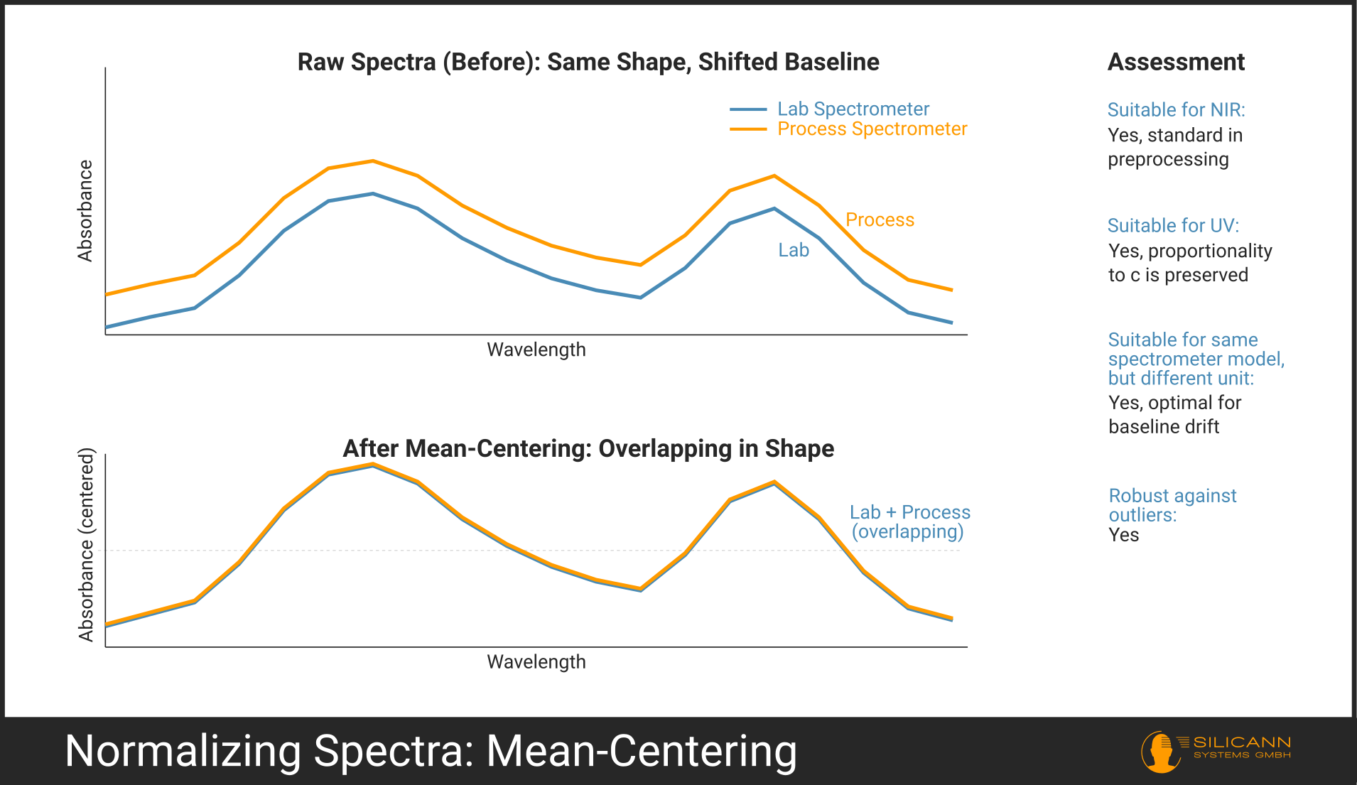
The method is robust because it does not use any single extreme value, but rather the mean of all measurement points. Outliers have only limited influence.
Vector Normalization: The Pure Shape
Vector normalization treats each spectrum as a vector in \(n\)-dimensional space (one dimension per wavelength) and divides by its Euclidean length:
\(X_{\text{norm}} = \frac{X}{\|X\|_2} = \frac{X}{\sqrt{\sum_{i=1}^{n} x_i^2}}\)
Each spectrum becomes a unit vector. With sklearn:
from sklearn.preprocessing import Normalizer

normalizer = Normalizer(norm='l2')
spectra_normalized = normalizer.fit_transform(spectra)
Instrument transfer: Vector normalization is the most powerful of the three tools - it eliminates both a constant offset and differing amplitudes between two instruments. After normalization, each spectrum lies on the same unit sphere; all that remains is the spectral direction. For two units of the same spectrometer type, this is almost always sufficient for successful calibration transfer.
UV vs. NIR use: Here the paths diverge. In NIR spectroscopy, vector normalization is a standard tool because NIR models rarely depend on absolute amplitudes; the wavelength ratios dominate. In UV spectrometry, vector normalization is only suitable for qualitative comparisons - for example, classification ("Is this substance A or B?"). For quantitative concentration determinations, it is unusable because the Beer-Lambert law \(A = \varepsilon \cdot c \cdot d\) requires a direct proportionality between absorbance height and concentration. Normalizing \(A\) to unit length destroys this proportionality. Vector normalization should therefore not be used in UV quantification.
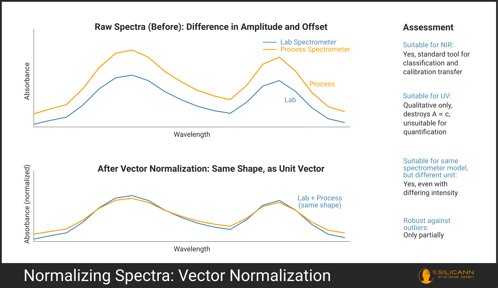
A side note on the risk of confusion: Vector normalization is conceptually similar to SNV (Standard Normal Variate), a classic of NIR preprocessing. However, SNV works pointwise (centres and divides by the standard deviation within the spectrum), whereas vector normalization treats the entire spectrum as a single unit.
Comparing the Three Methods
| Method | Corrects | Sensitivity | Same model, different unit? | UV (quantitative) | UV (qualitative) | NIR |
|---|---|---|---|---|---|---|
| Min-Max | Scales to [0,1] | Extreme: one outlier destroys everything | Yes, with similar dynamic range | No | Yes | Yes |
| Mean-Centering | Removes constant offset | Low: mean dampens outliers | Yes, optimal for baseline drift | Yes | Yes | Yes |
| Vector Norm | Removes offset + amplitude | Low to moderate | Yes, even with differing intensity | No | Yes | Yes |
The choice of method depends on three questions. First: do the instruments differ only in baseline offset? Then mean-centering suffices. Second: do they additionally differ in amplitude? Then vector normalization is needed - but only if UV quantification is not required. Third: are the spectra to serve as input for a neural network? Then Min-Max to \([0, 1]\) is the right choice, provided outliers have been removed beforehand.
Pitfalls in Practice
Some errors keep recurring when normalizing:
-
Normalization before the data split. The train/test split must occur before any normalization. Normalizing first and then splitting allows information from the test set to flow into the normalization parameters of the training set. This classic data leak then leads to overly optimistic RMSEP values. (More on this in the article on calibration and validation.)
-
Inconsistent normalization between lab and process. The normalization method with which the model was calibrated must be exactly the same as the one later applied to the process spectra. A model calibrated with mean-centering cannot interpret vector-normalized process data.
-
Vector normalization in UV quantification. As described in the previous section: whoever destroys \(A \propto c\) through normalization can no longer predict concentrations. This error can easily happen inadvertently when a measurement setup that previously only covered the NIR band is extended with a UV instrument to capture additional sample properties.
Summary
Transferring a lab calibration to process spectrometers can feel quite challenging at first glance. But carefully comparing the conditions at both locations already clears the most important hurdles. Spectra normalized using one of the methods described above are sufficient in most cases. Choosing the right method and applying it consistently between lab and process turns a lab calibration into a robust process model - with two units of the same spectrometer.
| Feature | Spektralwerk 15 Core NIR |
|---|---|
| Wavelength range | 900-1700 nm |
| Detector array | InGaAs, 256 pixels |
| Signal-to-noise ratio (SNR) | up to 10000:1 |
| Sample rate / spectra per second | > 500 Hz (streaming mode) |
| Trigger in and trigger out | yes |
| Spectral resolution (FWHM) | 3.9 nm (Hg line at 1014 nm) 5 nm (Hg line at 1529.6 nm) |
| Interfaces | Ethernet, FC (SMA on request) |
| Operating temperature | -5°C to +30°C |
| Ingress protection | IP40 (higher on request) |
| Details | Learn more |
Looking for an NIR spectrometry solution?
Thank you for your message!
We will get back to you as soon as possible.
Unfortunately, we were unable to transmit your message.
A technical error occured. Please try again later — or send an email to sales@silicann.com.
Thank you for your understanding.