Avoiding scattering errors in NIR spectroscopy

There is not only visible light, i.e. electromagnetic radiation with wavelengths between approx. 400 nm and 780 nm, but many more wavelength ranges that we can no longer see with our eyes. In the short-wave, higher-energy range, visible light is followed by UV radiation, and beyond the deep reds lies infrared radiation. We can't perceive UV radiation, but we can feel the infrared radiation as a thermal sensation through our skin. Visible light is used in sensing mainly for measurements of color and fluorescence. However, infrared radiation is of particular interest to spectrometry. It is so exciting because most molecules react to radiation in this wavelength range, and this reaction can be measured. Infrared radiation (IR radiation) is defined as wavelengths from 780 nm to 1,000,000 nm (1 mm). Within this range there are further subdivisions. The near infrared (NIR), with wavelengths from 780 nm to 2500 nm, is the part that directly adjoins visible light.

NIR spectroscopy: qualitative and quantitative

In NIR spectroscopy, one wants to make qualitative or quantitative statements about the sampled substance based on these reactions. Qualitative is a measurement if it can detect the presence of a substance (or its absence): What is this unknown sample? Is this substance at the goods receipt really the one we ordered? Are there impurities in this product? A quantitative measurement makes statements about the amount of a substance: How much protein is in these beans? How much omega-3 fatty acids are in that vegetable oil?

Whether pure or a mixture, in all these cases the samples consist of specific molecules. If such a sample is now irradiated with near-infrared, this means that photons with widely diverse wavelengths hit the sample. Since radiation with small wavelengths is more energetic than radiation with large wavelengths, the sample is hit by energy units of different sizes. Some of these energy units correspond exactly to the amount needed to make a certain molecule vibrate more strongly. In this case, this is exactly what happens: the energy of the photon is absorbed and converted into molecular motion (vibration of the atoms against each other, bending of the molecule, vibration of weakly bound molecules against each other). If one now measures the radiation with a spectrometer after contact with the sample, then exactly the photons that led to vibrations in the molecules will be missing. The wavelengths of these missing photons are the information that can be worked with in spectrometry: Each substance has a different molecular structure, and thus each has typical vibrations at very specific wavelengths. If exactly this combination is missing in the radiation after it has been in contact with the sample, then this is a sure sign of the presence of this specific molecule. And from the extent of the missing wavelengths, one can then also read off the proportion that this substance has in the sample.

Signal and noise

So much for the theory. In practice, we often have to deal with complex mixtures of substances. A vegetable oil consists of many different fatty acids whose overall chemical structure is quite similar. As a result, the typical absorption curves in each case will be partially superimposed. Quantitative measurements are even more challenging: the spectrum of rapeseed oil with 9% omega-3 content will be difficult to distinguish from that of a sample with 10% content. In the field, therefore, there is often a risk that the small variations between individual measurements may not be due to chemical differences between the individual samples at all, but perhaps should rather be explained by external interferences.

Some of the sources of error can be avoided by taking measurements that are as accurate as possible. A precise spectrometer is of course helpful, but a measurement setup that is as repeatable as possible is also important: For example, the measuring head should be at a constant distance from the samples. The same applies to extraneous light, i.e. sources of radiation in the production rooms that are not used to illuminate the sample. Ideally, the sample temperature is constant across all measurements, the surface and structure of the material being examined is always as identical as possible, the ambient temperature does not vary, etc. etc. In addition, the chemical analysis of the samples that is as precise as possible is important in advance. The content of the interesting substances in the sample is usually analyzed in the laboratory using classic chemical methods (however, in the case of common substances, this step is decades in the past, and a precise, already calibrated laboratory spectrometer is used instead). The results of these analyzes (the reference data) are then compared with spectral measurements so that it can be worked out mathematically which curves can be traced back to which ingredients. In the future, the spectral information will then be sufficient to determine the content of the ingredient.

But even when all these points have been diligently worked on, there will still be optical effects that overlay the chemical information in the spectrum, and in some cases even explain most of the differences between individual measurements. These optical effects are almost always scattering.

Reflection and refraction

Strictly speaking, scattering always occurs when electromagnetic waves hit matter: in this case, called elastic scattering, photons with the right energy are absorbed and re-emitted at the same time with identical wavelengths (this is a different process from that in which molecules are made to vibrate along their atomic bonds). At the macro level, elastic scattering can also be used to explain phenomena such as reflection and refraction, which are known from classical geometrical optics. In principle, this form of scattering is also not unimportant for spectrometry, because it leads to diffuse reflection.

Specular and diffuse reflection

In geometrical optics, an idealized situation is assumed: There is a solid material with a smooth surface, so that incoming light rays are reflected at exactly the angle at which they hit the surface. This is specular reflection. If we now zoom in to the site of the event at the atomic level, we see that the supposedly solid, smooth surface consists of nothing but molecules arranged more or less closely and systematically, with nothing between them. So it is not guaranteed that every photon takes the path of directed reflection. Instead, it can also be scattered inward into the sample, hit a molecule again, be scattered again, and only after a longer path through the material reach the outside again. This case is called diffuse reflection. In the case of specular reflection, there is practically no interaction between the material and the radiation. In this case, the radiation measured afterwards can contain almost no chemical information. Specular reflection can therefore superimpose the part of the radiation that contains the absorption signals sought, and is therefore interpreted in spectrometry as an interference factor and avoided as far as possible. Diffuse reflection is interesting from a measurement point of view, because here the radiation has penetrated the sample before being measured with the spectrometer. This will lead to absorption, so that the reflected radiation contains information about the structure of the material.

Undesired scattering effects in spectrometry

The scattering effects that lead to diffuse reflection are an essential basis for NIR spectroscopy. Other scattering effects are mainly sources of spurious noise that potentially obscure chemical information of interest.

Rayleigh scattering

Rayleigh scattering occurs when particles are significantly smaller than the wavelengths of the radiation (about 1/10 of the wavelength). This is true, for example, of visible sunlight and the atoms and molecules in our atmosphere. These particles do not have resonant frequencies in the wavelength range of visible light. If they are excited by a photon whith a wavelength significantly larger than themselves, then this is a case of elastic scattering: they absorb the photon, oscillate more strongly as a result, stop again at the same time and re-emit the photon with identical frequency/wavelength. The atoms are randomly oriented in the atmosphere, and therefore they will scatter the light randomly. However, the extent of the directional change also depends on the wavelength of the photon: The closer it is to the resonant frequency that each atom has in the UV region, the more the reemitted photon will deviate from its original direction. This is exactly what happens in our sky: The short wavelength blue light is much more likely to deviate from the original direction, to hit new atoms, to be scattered again - until it appears to us as terrestrial observers is if the entire sky was blue, because the scattered blue light hits our retina from every direction. Rayleigh radiation can also occur with larger objects, as long as the wavelengths then increase in the same ratio. In principle, Rayleigh scattering can also take place on tiny fibers, droplets or bubbles, as long as the wavelength of the incident radiation is at least ten times the diameter of these particles. The shape of the particles is of little importance.

Mie scattering

The more the particle size approaches the wavelength, the less the observable phenomena can be explained by Rayleigh scattering. As soon as the wavelengths are approximately equal to the particle diameter and the particles are roughly spherical, we are in Mie scattering terrain. In this region, the scattering is much less wavelength dependent. Again, this can be seen in the sky, because Mie scattering is the reason why clouds look so gray. The tiny water droplets are roughly round and about equal in size to the wavelength of visible light. As a result, the sun's light rays are refracted by them regardless of wavelength. All the color components originally contained in the sunlight are thus preserved, but they are partially scattered away from our eye, so that this part of the sky appears darker. If the particles become significantly larger than the wavelengths, again by a factor of about 10, then we leave the Mie scattering range. From this moment on, the effects can be predicted well by the means of geometrical optics. In the near-infrared range, it is not at all unlikely to be directly confronted with Mie scattering during spectrometric measurements. Smallest fibers, fat droplets, air bubbles or similar particles with diameters of 1-3 µm may well be present in the samples investigated with NIR spectrometers.

This is problematic for precise results, because these scattering effects will lead to altered spectra: Now we no longer only have absorption as a reason why less radiation is measured at certain wavelengths, but also scattering effects.

Spectral preprocessing

Historically, this physical obfuscation of the chemical signal was indeed a limitation that initially prevented the productive use of NIR spectroscopy. Only the mathematical processing of the spectra with the help of computers brought progress here.

Derivatives

The first and still used form of pre-processing was the derivation. Derivatives emphasize the peaks in spectra. Higher derivations can also separate peaks that have arisen by superimposing the individual peaks of different substances. In the first derivative, a peak in an absorption spectrum swings up to a maximum just before and a correspondingly mirrored minimum just after the original peak, so that the position of the original peak is exactly 0. The second derivative leads to a minimum where there was a maximum in the unprocessed spectrum. This derivation is probably used most frequently in practice.

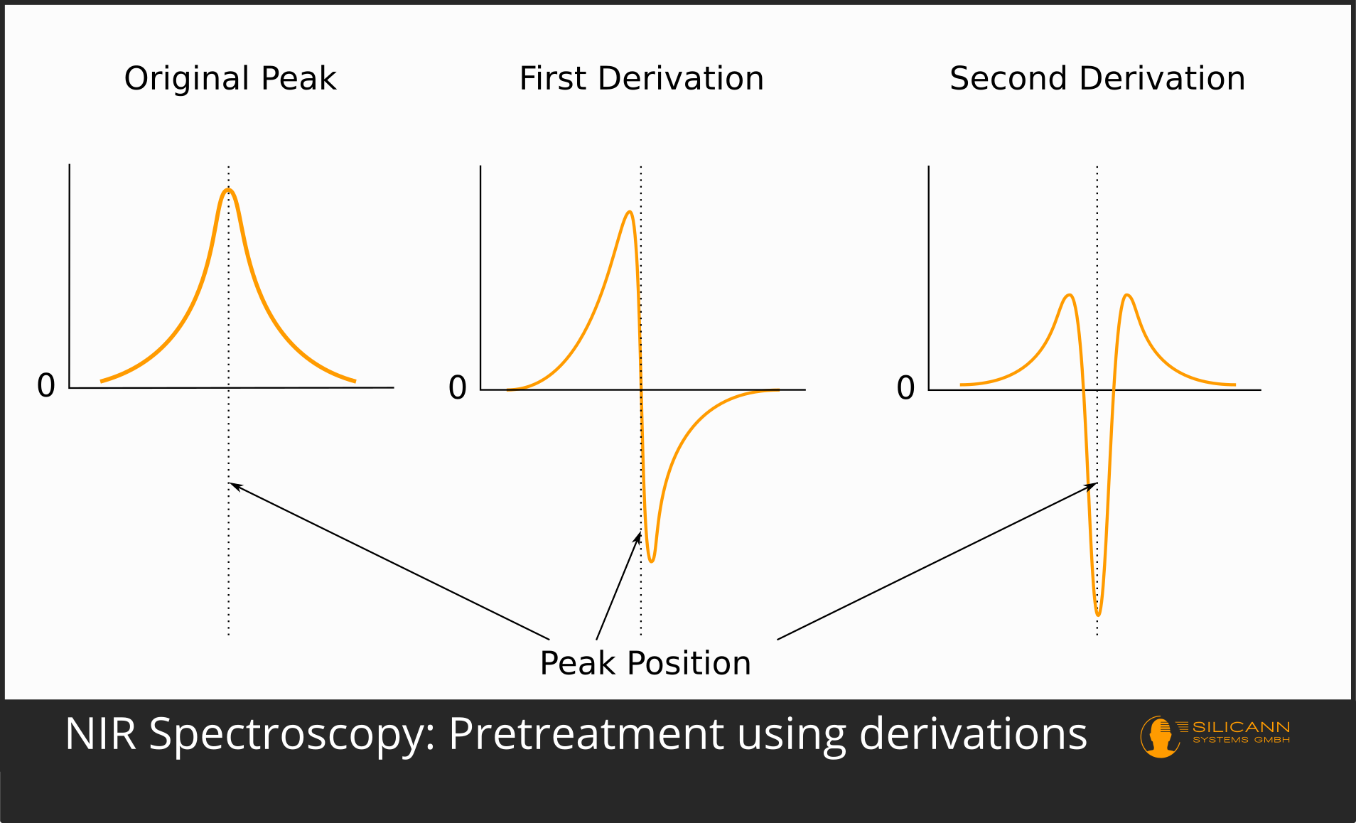
The use of the third and fourth derivative is also not uncommon. However, it is true that using higher derivatives is also more likely to introduce artifacts that artificially invent peaks that were not present in the actual spectrum. A very commonly used algorithm is Savitzky-Golay.

Derivatives work on a single spectrum, unrelated to the other spectra in the measurement series.

MSC: Multiplicative Scatter Correction

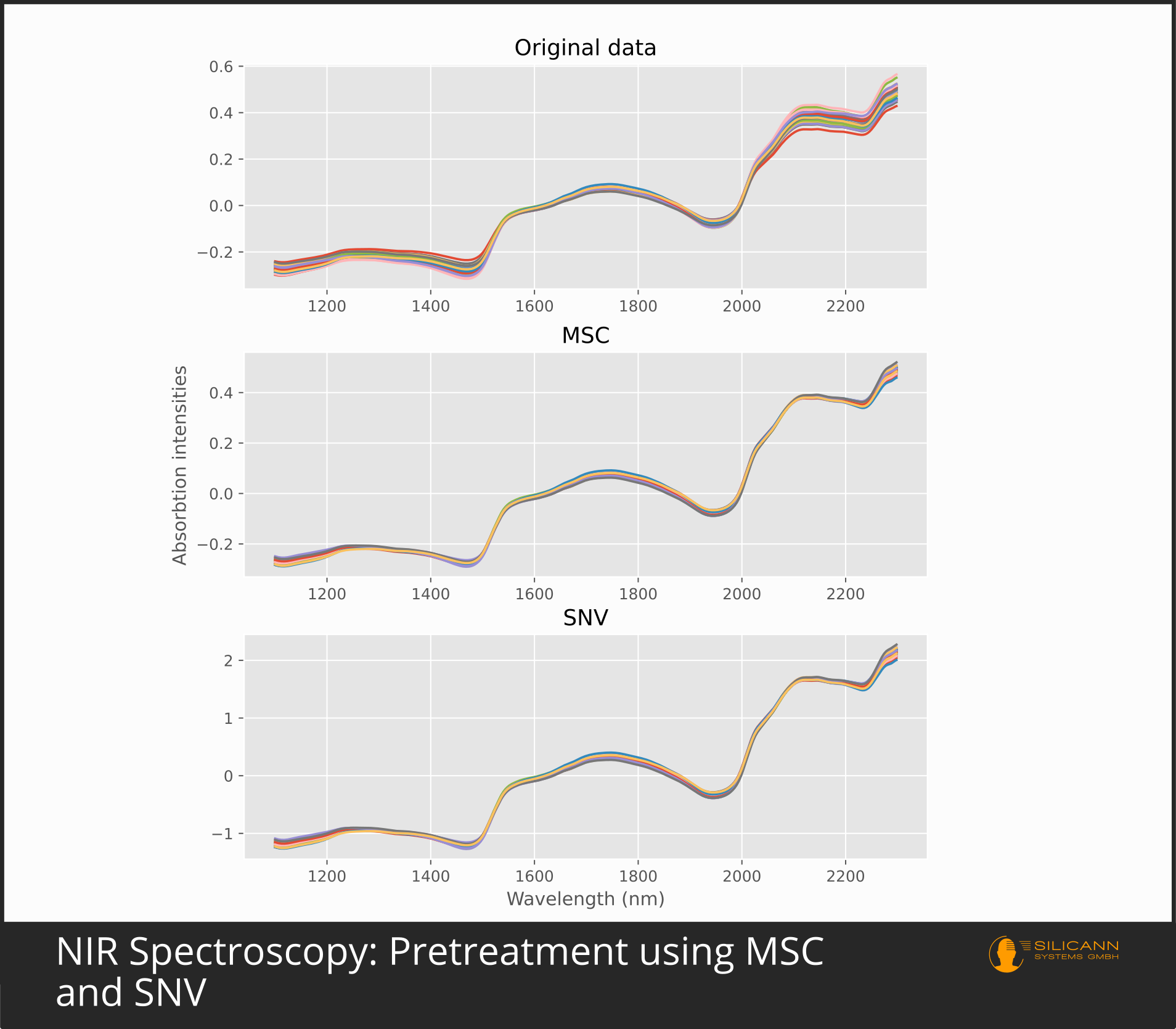
This is different with Multiplicative Scatter Correction. MSC is designed to separate signal from noise for both additive and multiplicative errors. Additive errors are constant scattering errors. In a spectrum, they would result in all values being shifted up or down by a certain factor along the y-axis, the axis signifying the intensities. A possible reason for this would be path length differences caused by scattering. Multiplicative errors cause the spectrum to tilt so that the values increase as we get further into the long-wavelength region of the x-axis, the wavelength axis. This type of error is caused, for example, by Mie scattering on small particles that are of this scale. The basis of how multiplicative scatter correction works is the observation that the scattering effects, e.g. caused by this Mie scattering, have a different wavelength dependence than the absorption effects that result from the chemical nature of the sample. The actually measured spectrum should be compared with the ideal spectrum of the sample, a spectrum without any kind of scattering error. Such an ideal spectrum is difficult to obtain in practice, which is why the path from the original paper is almost always taken in practice: an average spectrum is calculated from many different measurements of very similar samples and used as a substitute for the ideal spectrum. Internally, a and b are then calculated using least squares regression for the following formula:

X = a + b*X' + E

Here X is the concrete spectrum, X' is the ideal spectrum, a is the additive component (i.e. the additive error, the shift along the y-axis) and b is the multiplicative component (the slope around the intersection with the y-axis). E corresponds to the residual spectrum, which then ideally only contains chemical information. The intercept and slope are calculated so that the concrete spectrum and the averaged spectrum start with the same absorption at the shortest wavelength and have the same slope as the wavelength progresses. Since the publication of the introductory paper in 1985, MSC has been used very frequently as a preprocessing step, especially in combination with PLS as a calibration method. In the meantime, there are also various extensions of this approach, which can then, in particular, compensate for more complex, nonlinear scattering.

SNV: Standard Normal Variate Transformation

The preprocessing variant Standard Normal Variate (SNV) is used for similar situations as MSC: as a means against scatter and for scenarios with varying path length to the sample. Accordingly, it can also be used to compensate for differently rough sample surfaces, because that is synonymous to different particle sizes, and thus again (Mie) scattering effects. In contrast to MSC, however, the correction with SNV is only based on the individual, concrete spectrum. The authors of the paper justify this with the fact that the multiplicative scattering effects have their cause in the respective individual sample (e.g. in the individually different surface properties), not in the totality of all samples, and therefore only the individual spectrum must be used for a correction. SNV reduces the error part of the spectral intensities by taking the mean value of all intensities, subtracting it from all individual values and then dividing it by the standard deviation. After applying SNV, the resulting spectrum usually still has a clearly visible increasing trend towards longer wavelengths. To counter this, the authors have proposed detrending using a second degree polynomial.

MSC or SNV?

In practice, MSC and SNV in NIR spectroscopy generally give comparable results. Which approach is to be given preference and whether the second derivation is sufficient depends heavily on the specific samples and the measurement conditions. Since derivations primarily emphasize the peaks and MSC, SNV and similar algorithms primarily reduce errors, there is nothing principally wrong with the simultaneous use of both approaches.

The pre-processing of the spectrum is usually followed by the calibration, i.e. the attempt to be able to predict the chemical information from the optical signal. In case of doubt, the decision on the preprocessing method should be based on the resulting prediction error of this calibration.

Quellen

• Hecht: Optics, 5th edition, 2017
• Geladi, MacDougall, Martens: Linearization and Scatter-Correction for Near-Infrared Reflectance Spectra of Meat, 1985
• Barnes, Dhanoa, Lister: Standard Normal Variate Transformation and De-trending of Near-Infrared Diffuse Reflectance Spectra, 1989